7. Utilities for observations handling

In previous notebooks, the xs.spatial.subset and xs.spatial_mean methods have already been shown, but xscen ships with a few more spatial utilities and other functions that come handy when handling observations (point timeseries).

[1]:

import numpy as np
import xarray as xr
import xclim as xc
import xscen as xs

import string
import random

import cartopy.crs as ccrs
import cartopy.feature as cfeat
import matplotlib.pyplot as plt

Let’s first create synthetic data for the example. We have here one year of daily tas data on a 50x50 grid with a Rotated Pole projection. We also have the same year of tas data at 102 “stations”.

[2]:

ds = xs.testing.datablock_3d(np.random.random((366, 50, 50)), "tas", "rlon", -25, "rlat", -25, 1, 1, "2000-01-01", as_dataset=True)

[3]:

N = 100
obs = xc.testing.helpers.test_timeseries(np.random.random(366,), 'tas', start='2000-01-01', as_dataset=True)
stations = ['00', '01'] + [''.join(random.choices(string.ascii_letters, k=4)) for i in range(N)]
lon = [-100, -100] + list(np.random.randint(-120, -60, size=N))
lat = [45, 45] + list(np.random.randint(30, 60, size=N))
obs = obs.expand_dims(station=stations).assign_coords(lon=(('station',), lon), lat=(('station',), lat))
obs

7.2. Voronoi weights

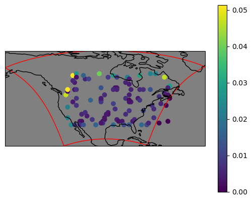
When comparing observations to gridded data, one often averages some statistics over multiple stations. When done without weighting, this average treats all stations as equal, which implictely gives a stronger weight to regions with many stations. This is not always wanted. Voronoi weights are a way to enhance the geographical representativity of the average by giving less weight to stations in densely observed areas. The process divides an area with small polygons in such a way that each polygon includes exactly one station. The weights are then the fraction of the total area covered by this polygon. Further info is available on Wikipedia.

The xscen function does not store the polygons, it only returns the weight.

Here, we limit the voronoi polygon to the total extent of the dataset (using another handy xscen function). We could also pass a GeoDataFrame with a collection of polygons so that the weights are computed for each region. One can see in the figure that stations outside the region were attributed a weight of 0. We also limit the maximum weight to 5% (0.05) in order to lessen the impact of outlier stations.

[5]:

extent = xs.spatial.dataset_extent(ds, method='shape')
vw = xs.spatial.voronoi_weights(obs, region=extent['shape'], maxfrac=0.05)
obs = obs.assign_coords(weight=vw)

[6]:

fig, ax = plt.subplots(subplot_kw={'projection': ccrs.PlateCarree()})
sc = ax.scatter(x=obs.lon, y=obs.lat, c=obs.weight, transform=ccrs.PlateCarree())
ax.add_geometries([extent['shape']], facecolor='none', edgecolor='red', crs=ccrs.PlateCarree())
ax.coastlines()
ax.set_facecolor('grey')
bs = extent['shape'].bounds
ax.set_extent([bs[0], bs[2], bs[1], bs[3]], crs=ccrs.PlateCarree())
fig.colorbar(sc)

[6]:

<matplotlib.colorbar.Colorbar at 0x7a10389ec590>

/home/docs/checkouts/readthedocs.org/user_builds/xscen/conda/latest/lib/python3.13/site-packages/cartopy/io/__init__.py:242: DownloadWarning: Downloading: https://naturalearth.s3.amazonaws.com/110m_physical/ne_110m_coastline.zip

../_images/notebooks_7_spatial_utils_9_2.png

If we computed some RSME, for example, we could do the average with:

[7]:

ds_at_obs = xs.spatial.subset(ds, 'gridpoint', lon=obs.lon, lat=obs.lat)
rmse = ((ds_at_obs.tas - obs.tas)**2).mean('time')**0.5
rmse.weighted(obs.weight).mean()

[7]:

<xarray.DataArray 'tas' ()> Size: 8B
array(0.41541387)
Coordinates:
    rotated_pole  <U1 4B ''

7. Utilities for observations handling

7.1. Merge colocated stations

7.2. Voronoi weights