4. Ensembles

4.1. Ensemble reduction

This tutorial will explore ensemble reduction (also known as ensemble selection) using xscen. This will use pre-computed annual mean temperatures from xclim.testing.

from xclim.testing import open_dataset

import xscen as xs

datasets = {
    "ACCESS": "EnsembleStats/BCCAQv2+ANUSPLIN300_ACCESS1-0_historical+rcp45_r1i1p1_1950-2100_tg_mean_YS.nc",
    "BNU-ESM": "EnsembleStats/BCCAQv2+ANUSPLIN300_BNU-ESM_historical+rcp45_r1i1p1_1950-2100_tg_mean_YS.nc",
    "CCSM4-r1": "EnsembleStats/BCCAQv2+ANUSPLIN300_CCSM4_historical+rcp45_r1i1p1_1950-2100_tg_mean_YS.nc",
    "CCSM4-r2": "EnsembleStats/BCCAQv2+ANUSPLIN300_CCSM4_historical+rcp45_r2i1p1_1950-2100_tg_mean_YS.nc",
    "CNRM-CM5": "EnsembleStats/BCCAQv2+ANUSPLIN300_CNRM-CM5_historical+rcp45_r1i1p1_1970-2050_tg_mean_YS.nc",
}

for d in datasets:
    ds = open_dataset(datasets[d]).isel(lon=slice(0, 4), lat=slice(0, 4))
    ds = xs.climatological_op(
        ds,
        op="mean",
        window=30,
        periods=[[1981, 2010], [2021, 2050]],
        horizons_as_dim=True,
    ).drop_vars("time")
    datasets[d] = xs.compute_deltas(ds, reference_horizon="1981-2010")

ERROR 1: PROJ: proj_create_from_database: Open of /home/docs/checkouts/readthedocs.org/user_builds/xscen/conda/latest/share/proj failed

4.1.1. Preparing the data

Ensemble reduction is built upon climate indicators that are relevant to represent the ensemble’s variability for a given application. In this case, we’ll use the mean temperature delta between 2021-2050 and 1981-2010, but monthly or seasonal indicators could also be required. The horizons_as_dim argument in climatological_op can help combine indicators of multiple frequencies into a single dataset. Alternatively, xscen.utils.unstack_dates can also accomplish the same thing if the climatological operations have already been computed.

The functions implemented in xclim.ensembles._reduce require a very specific 2-D DataArray of dimensions “realization” and “criteria”. The first solution is to first create an ensemble using xclim.ensembles.create_ensemble, then pass the result to xclim.ensembles.make_criteria. Alternatively, the datasets can be passed directly to xscen.ensembles.reduce_ensemble and the necessary preliminary steps will be accomplished automatically.

In this example, the number of criteria will corresponds to: indicators x horizons x longitude x latitude, but criteria that are purely NaN across all realizations will be removed.

Note that xs.spatial_mean could have been used prior to calling that function to remove the spatial dimensions.

4.1.2. Selecting a reduced ensemble

NOTE

Ensemble reduction in xscen is built upon xclim.ensembles. For more information on basic usage and available methods, please consult their documentation.

Ensemble reduction through xscen.reduce_ensemble consists in a simple call to xclim. The arguments are: - data, which is the aforementioned 2D DataArray, or the list/dict of datasets required to build it. - method is either kkz or kmeans. See the link above for further details on each technique. - horizons is used to instruct on which horizon(s) to build the data from, if data needs to be constructed. - create_kwargs, the arguments to pass to xclim.ensembles.create_ensemble if data needs to be constructed. - kwargs is a dictionary of arguments to send to the clustering method chosen.

selected, clusters, fig_data = xs.reduce_ensemble(
    data=datasets, method="kmeans", horizons=["2021-2050"], max_clusters=3
)

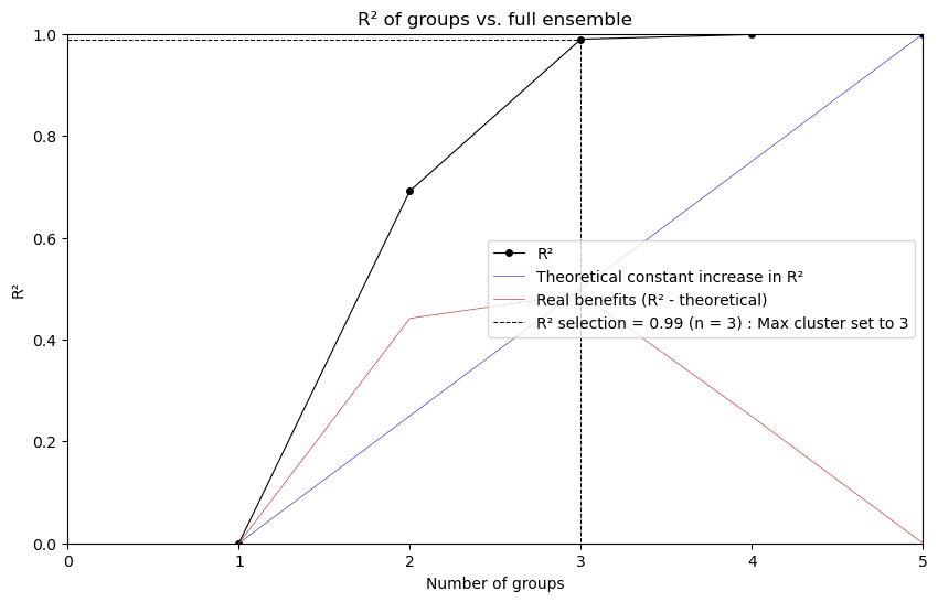
The method always returns 3 outputs (selected, clusters, fig_data): - selected is a DataArray of dimension ‘realization’ listing the selected simulations. - clusters (kmeans only) groups every realization in their respective clusters in a python dictionary. - fig_data (kmeans only) can be used to call xclim.ensembles.plot_rsqprofile(fig_data)

selected

<xarray.DataArray 'realization' (realization: 3)> Size: 96B
array(['ACCESS', 'BNU-ESM', 'CNRM-CM5'], dtype='<U8')
Coordinates:
  * realization  (realization) <U8 96B 'ACCESS' 'BNU-ESM' 'CNRM-CM5'
Attributes:
    axis:     E

xarray.DataArray

'realization'

• realization: 3

• 'ACCESS' 'BNU-ESM' 'CNRM-CM5'

  array(['ACCESS', 'BNU-ESM', 'CNRM-CM5'], dtype='<U8')

• Coordinates: (1)
  • realization
    (realization)
    <U8
    'ACCESS' 'BNU-ESM' 'CNRM-CM5'

    axis :

    E

    array(['ACCESS', 'BNU-ESM', 'CNRM-CM5'], dtype='<U8')

• Indexes: (1)
  • realization
    PandasIndex

    PandasIndex(Index(['ACCESS', 'BNU-ESM', 'CNRM-CM5'], dtype='object', name='realization'))

• Attributes: (1)

  axis :

  E

# To see the clusters in more details
clusters

{0: <xarray.DataArray 'realization' (realization: 3)> Size: 96B
 array(['ACCESS', 'CCSM4-r1', 'CCSM4-r2'], dtype='<U8')
 Coordinates:
   * realization  (realization) <U8 96B 'ACCESS' 'CCSM4-r1' 'CCSM4-r2'
 Attributes:
     axis:     E,
 1: <xarray.DataArray 'realization' (realization: 1)> Size: 32B
 array(['BNU-ESM'], dtype='<U8')
 Coordinates:
   * realization  (realization) <U8 32B 'BNU-ESM'
 Attributes:
     axis:     E,
 2: <xarray.DataArray 'realization' (realization: 1)> Size: 32B
 array(['CNRM-CM5'], dtype='<U8')
 Coordinates:
   * realization  (realization) <U8 32B 'CNRM-CM5'
 Attributes:
     axis:     E}

from xclim.ensembles import plot_rsqprofile

plot_rsqprofile(fig_data)

4.2. Ensemble partition

This tutorial will show how to use xscen to create the input for xclim partition functions.

# Get catalog
from pathlib import Path

output_folder = Path().absolute() / "_data"
cat = xs.DataCatalog(str(output_folder / "tutorial-catalog.json"))

# create a dictionnary of datasets wanted for the partition
input_dict = cat.search(variable="tas", member="r1i1p1f1").to_dataset_dict(
    xarray_open_kwargs={"engine": "h5netcdf"}
)

--> The keys in the returned dictionary of datasets are constructed as follows:
        'id.domain.processing_level.xrfreq'

100.00% [4/4 00:00<00:00]

From a dictionary of datasets, the function creates a dataset with new dimensions in partition_dim(["source", "experiment", "bias_adjust_project"], if they exist). In this toy example, we only have different experiments. - By default, it translates the xscen vocabulary (eg. experiment) to the xclim partition vocabulary (eg. scenario). It is possible to pass rename_dict to rename the dimensions with other names. - If the inputs are not on the same grid, they can be regridded through regrid_kw or subset to a point through subset_kw. The functions assumes that if there are different bias_adjust_project, they will be on different grids (with all source on the same grid). If there is one or less bias_adjust_project, the assumption is thatsource have different grids. - You can also compute indicators on the data if the input is daily. This can be especially useful when the daily input data is on different calendars.

# build a single dataset
import xclim as xc

ds = xs.ensembles.build_partition_data(
    input_dict,
    subset_kw=dict(name="mtl", method="gridpoint", lat=[45.5], lon=[-73.6]),
    indicators_kw={"indicators": [xc.atmos.tg_mean]},
)
ds

<xarray.Dataset> Size: 220B
Dimensions:   (time: 2, scenario: 4, model: 1)
Coordinates:
  * time      (time) datetime64[ns] 16B 2001-01-01 2002-01-01
  * scenario  (scenario) object 32B 'ssp126' 'ssp245' 'ssp370' 'ssp585'
  * model     (model) <U23 92B 'NCC_NorESM2-MM_r1i1p1f1'
    lat       float64 8B 45.0
    lon       int64 8B -74
Data variables:
    tg_mean   (scenario, model, time) float64 64B dask.array<chunksize=(4, 1, 2), meta=np.ndarray>
Attributes: (12/22)
    comment:                 This is a test file created for the xscen tutori...
    version:                 v20191108
    intake_esm_vars:         ['tas']
    cat:id:                  CMIP6_ScenarioMIP_NCC_NorESM2-MM_ssp370_r1i1p1f1...
    cat:type:                simulation
    cat:processing_level:    indicators
    ...                      ...
    cat:date_start:          2001-01-01 00:00:00
    cat:date_end:            2002-12-31 00:00:00
    cat:_data_format_:       nc
    cat:path:                /home/docs/checkouts/readthedocs.org/user_builds...
    intake_esm_dataset_key:  CMIP6_ScenarioMIP_NCC_NorESM2-MM_ssp370_r1i1p1f1...
    history:                 [2024-04-26 15:27:36] gridpoint spatial subsetti...

xarray.Dataset

• Dimensions:
  • time: 2
  • scenario: 4
  • model: 1
• Coordinates: (5)
  • time
    (time)
    datetime64[ns]
    2001-01-01 2002-01-01

    array(['2001-01-01T00:00:00.000000000', '2002-01-01T00:00:00.000000000'],
          dtype='datetime64[ns]')

  • scenario
    (scenario)
    object
    'ssp126' 'ssp245' 'ssp370' 'ssp585'

    array(['ssp126', 'ssp245', 'ssp370', 'ssp585'], dtype=object)

  • model
    (model)
    <U23
    'NCC_NorESM2-MM_r1i1p1f1'

    array(['NCC_NorESM2-MM_r1i1p1f1'], dtype='<U23')

  • lat
    ()
    float64
    45.0

    units :

    degrees_north

    description :

    Latitude.

    standard_name :

    latitude

    axis :

    Y

    array(45.)

  • lon
    ()
    int64
    -74

    units :

    degrees_east

    description :

    Longitude.

    standard_name :

    longitude

    axis :

    X

    array(-74)

• Data variables: (1)
  • tg_mean
    (scenario, model, time)
    float64
    dask.array<chunksize=(4, 1, 2), meta=np.ndarray>

    description :

    Annual mean of daily mean temperature.

    standard_name :

    air_temperature

    cell_methods :

    time: mean time: mean over days

    units :

    K

    history :

    [2024-04-26 15:27:36] tg_mean: TG_MEAN(tas=tas, freq='YS') with options check_missing=any - xclim version: 0.48.2

    long_name :

    Mean daily mean temperature

    Array Chunk Bytes 64 B 64 B Shape (4, 1, 2) (4, 1, 2) Dask graph 1 chunks in 96 graph layers Data type float64 numpy.ndarray

• Indexes: (3)
  • time
    PandasIndex

    PandasIndex(DatetimeIndex(['2001-01-01', '2002-01-01'], dtype='datetime64[ns]', name='time', freq='YS-JAN'))

  • scenario
    PandasIndex

    PandasIndex(Index(['ssp126', 'ssp245', 'ssp370', 'ssp585'], dtype='object', name='scenario'))

  • model
    PandasIndex

    PandasIndex(Index(['NCC_NorESM2-MM_r1i1p1f1'], dtype='object', name='model'))

• Attributes: (22)

  comment :

  This is a test file created for the xscen tutorial. This file is not a real CMIP6 file.

  version :

  v20191108

  intake_esm_vars :

  ['tas']

  cat:id :

  CMIP6_ScenarioMIP_NCC_NorESM2-MM_ssp370_r1i1p1f1_example-region

  cat:type :

  simulation

  cat:processing_level :

  indicators

  cat:mip_era :

  CMIP6

  cat:activity :

  ScenarioMIP

  cat:institution :

  NCC

  cat:source :

  NorESM2-MM

  cat:experiment :

  ssp370

  cat:member :

  r1i1p1f1

  cat:xrfreq :

  YS-JAN

  cat:frequency :

  yr

  cat:variable :

  ('tg_mean',)

  cat:domain :

  mtl

  cat:date_start :

  2001-01-01 00:00:00

  cat:date_end :

  2002-12-31 00:00:00

  cat:_data_format_ :

  nc

  cat:path :

  /home/docs/checkouts/readthedocs.org/user_builds/xscen/checkouts/latest/docs/notebooks/_data/path_builder_examples/simulation/raw/CMIP6/ScenarioMIP/example-region/NCC/NorESM2-MM/ssp370/r1i1p1f1/day/tas/tas_day_CMIP6_ScenarioMIP_example-region_NCC_NorESM2-MM_ssp370_r1i1p1f1_2001-2002.nc

  intake_esm_dataset_key :

  CMIP6_ScenarioMIP_NCC_NorESM2-MM_ssp370_r1i1p1f1_example-region.example-region.raw.D

  history :

  [2024-04-26 15:27:36] gridpoint spatial subsetting on 1 coordinates - clisops v0.13.0

Pass the input to an xclim partition function.

# compute uncertainty partitionning
mean, uncertainties = xc.ensembles.hawkins_sutton(ds.tg_mean)
uncertainties

<xarray.DataArray (uncertainty: 4, time: 4)> Size: 128B
dask.array<concatenate, shape=(4, 4), dtype=float64, chunksize=(1, 2), chunktype=numpy.ndarray>
Coordinates:
    lat          float64 8B 45.0
    lon          int64 8B -74
  * time         (time) object 32B 2001-01-01 00:00:00 ... 2004-01-01 00:00:00
  * uncertainty  (uncertainty) object 32B 'variability' 'model' ... 'total'
Attributes:
    model:     ['NCC_NorESM2-MM_r1i1p1f1']
    scenario:  ['ssp126' 'ssp245' 'ssp370' 'ssp585']

xarray.DataArray

• uncertainty: 4
• time: 4

• dask.array<chunksize=(1, 2), meta=np.ndarray>

  Array Chunk Bytes 128 B 16 B Shape (4, 4) (1, 2) Dask graph 8 chunks in 218 graph layers Data type float64 numpy.ndarray

• Coordinates: (4)
  • lat
    ()
    float64
    45.0

    array(45.)

  • lon
    ()
    int64
    -74

    array(-74)

  • time
    (time)
    object
    2001-01-01 00:00:00 ... 2004-01-...

    array([cftime.DatetimeGregorian(2001, 1, 1, 0, 0, 0, 0, has_year_zero=False),
           cftime.DatetimeGregorian(2002, 1, 1, 0, 0, 0, 0, has_year_zero=False),
           cftime.DatetimeGregorian(2003, 1, 1, 0, 0, 0, 0, has_year_zero=False),
           cftime.DatetimeGregorian(2004, 1, 1, 0, 0, 0, 0, has_year_zero=False)],
          dtype=object)

  • uncertainty
    (uncertainty)
    object
    'variability' 'model' ... 'total'

    array(['variability', 'model', 'scenario', 'total'], dtype=object)

• Indexes: (2)
  • time
    PandasIndex

    PandasIndex(CFTimeIndex([2001-01-01 00:00:00, 2002-01-01 00:00:00, 2003-01-01 00:00:00,
                 2004-01-01 00:00:00],
                dtype='object', length=4, calendar='standard', freq='YS-JAN'))

  • uncertainty
    PandasIndex

    PandasIndex(Index(['variability', 'model', 'scenario', 'total'], dtype='object', name='uncertainty'))

• Attributes: (2)

  model :

  ['NCC_NorESM2-MM_r1i1p1f1']

  scenario :

  ['ssp126' 'ssp245' 'ssp370' 'ssp585']

NOTE

Note that the figanos library provides a function fg.partition to plot the uncertainties.